The sxts (spatial xts) class

library(anyFit)
library(xts)
library(ggplot2)
library(patchwork)

1. What is an `sxts`?

Gridded hydroclimatic data are two things at once: a time series (many time steps) and a spatial field (many locations). Workflows that maintain these separately, a raster for space and an xts for time, incur both a memory overhead and the constant risk of the two representations drifting out of alignment.

anyFit’s answer is the sxts (spatial xts) class. It is a lightweight S3 extension of xts: the data matrix has one row per time step and one column per grid cell, and three pieces of spatial metadata are carried as attributes:

coords: a data frame of x/y coordinates, one row per column of data;
projection: a CRS string describing the coordinate reference system;
elements: the number of spatial locations (i.e. data columns).

Because sxts extends xts rather than replacing it, the entire xts toolbox (temporal subsetting, period aggregation, date arithmetic) remains available, while the spatial context is retained through every operation.

2. Constructing an `sxts`

The usual way to obtain one is to read a NetCDF file with nc2xts(), which returns an sxts directly. We use the bundled E-OBS daily rainfall file, clipped to the UK.

f <- system.file("extdata", "rr_ens_mean_0.25deg_reg_2011-2022_v27.0e.nc",
                 package = "anyFit")
uk_name <- "U.K. of Great Britain and Northern Ireland"

rain_uk <- nc2xts(f, varname = "rr", country = uk_name)

The dedicated str() and summary() methods report the spatial and temporal extent concisely:

str(rain_uk)
#> 'sxts' Spatial xts object
#>  Description:  This is a spatial xts (sxts) object 
#>  Projection:  +proj=longlat +datum=WGS84 
#>  Elements:  544  spatial locations
#> Spatial extent is: -7.875 , 1.625 , 50.125 , 60.625  (xmin, xmax, ymin, ymax) 
#>  Time series data:
#> Range of dates is from: 2011-01-01 to: 2022-12-31

You can also build an sxts from scratch with the sxts() constructor, passing a data matrix, a time index, a coordinate table and a projection, which is useful when the data do not come from NetCDF. The constructor validates that the number of coordinate rows matches the number of data columns.

set.seed(1)
dates  <- seq(as.POSIXct("2020-01-01", tz = "UTC"), by = "day", length.out = 30)
coords <- data.frame(x = c(-2, -1, 0), y = c(51, 52, 53))
vals   <- matrix(rgamma(30 * 3, shape = 1, scale = 3), nrow = 30, ncol = 3)

toy <- sxts(vals, order.by = dates, coords = coords,
            projection = "+proj=longlat +datum=WGS84")
is.sxts(toy)
#> [1] TRUE

3. Accessing spatial metadata

Three accessor functions expose the spatial attributes:

elements(rain_uk)          # number of grid cells
#> [1] 544
projection(rain_uk)        # coordinate reference system
#> [1] "+proj=longlat +datum=WGS84"
head(coords(rain_uk))      # x / y coordinates, one row per cell
#>          x      y
#> 54  -5.625 50.125
#> 55  -5.375 50.125
#> 56  -5.125 50.125
#> 99  -4.875 50.375
#> 100 -4.625 50.375
#> 101 -4.375 50.375

4. Subsetting is spatially aware

The [ method treats the two dimensions differently. Subsetting by time (rows), using the full range of xts date-string syntax, retains every location:

winter15 <- rain_uk["2015-12"]     # December 2015, all cells
c(rows = nrow(winter15), cells = elements(winter15))
#>  rows cells 
#>    31   544

Subsetting by location (columns) updates the stored coordinates and the element count to match, so that the metadata remains consistent with the data:

first_ten <- rain_uk[, 1:10]
c(cells = elements(first_ten), coord_rows = nrow(coords(first_ten)))
#>      cells coord_rows 
#>         10         10

5. Arithmetic, lagging and differencing preserve the class

Element-wise arithmetic, comparison, lag() and diff() all return an sxts with the spatial attributes preserved automatically:

rain_cm <- rain_uk / 10          # mm -> cm
is.sxts(rain_cm)
#> [1] TRUE

lagged <- lag(rain_uk, 1)        # one-day lag, still an sxts
is.sxts(lagged)
#> [1] TRUE

6. Spatial operations native to `sxts`

Masking

mask.sxts() restricts an sxts to a region, given as a bounding box, a shapefile, or an sf/Spatial* object. Here we crop to a box over central England and confirm that the cell count is reduced.

box <- mask.sxts(rain_uk, xlim = c(-3, 0), ylim = c(51.5, 53.5))
elements(box)
#> [1] 95

nc_ggplot(basic_stats_nc(box)[["Mean"]], legend.title = "Mean (mm)",
          viridis.option = "mako") +
  borders("world", regions = "UK")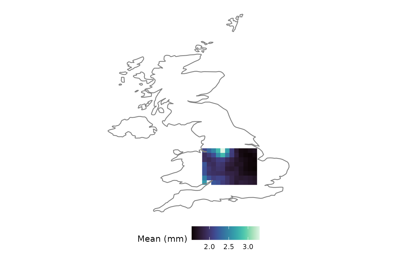

Zonal statistics

zonal_stats() collapses the spatial dimension by aggregating all cells that fall within one or more polygons (supplied as a shapefile, a country or a continent) and returns a plain xts with one column per polygon. Below we compute the daily spatial-mean rainfall over the UK, then aggregate it to monthly totals for a readable series. Because the E-OBS grid contains some missing cells, we supply an na.rm = TRUE mean, so that a single missing cell does not propagate to the entire day.

uk_mean_daily <- zonal_stats(rain_uk, country = uk_name,
                             FUN = function(x) mean(x, na.rm = TRUE))
uk_monthly <- aggregate_xts(uk_mean_daily, periods = "months",
                            FUN = "sum")$list_months$aggregated

autoplot(uk_monthly) +
  labs(y = "UK mean rainfall (mm/month)", x = NULL) +
  theme_bw()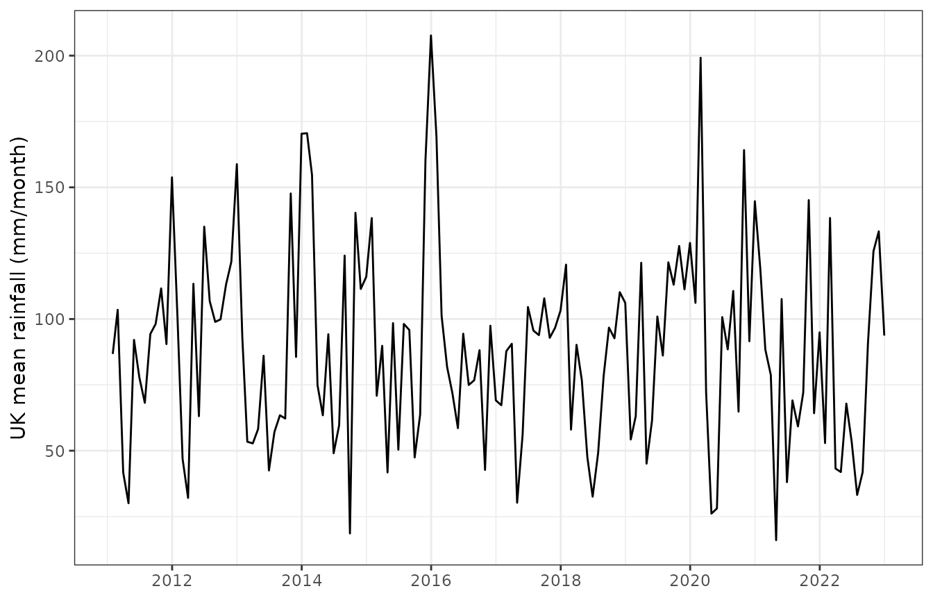

Conversion to and from rasters

When data must be passed to a raster-based tool, rasterFromSxts() produces a RasterBrick with time as the z-dimension, and sxtsFromRaster() performs the inverse conversion. The round trip is lossless for the data and reconstructs the spatial metadata.

brick_uk <- rasterFromSxts(rain_uk)
class(brick_uk)
#> [1] "RasterBrick"
#> attr(,"package")
#> [1] "raster"

back <- sxtsFromRaster(brick_uk)
c(is_sxts = is.sxts(back), cells = elements(back))
#> is_sxts   cells 
#>       1     499

7. Concatenating along time

Reading a multi-file dataset produces a list of sxts objects that share a grid. rbindlist.sxts() concatenates them into one continuous series in a single pass, which is considerably faster than repeated pairwise rbind. To illustrate, we split the UK series into two by time and recombine it.

part1 <- rain_uk["2011/2016"]
part2 <- rain_uk["2017/2022"]

recombined <- rbindlist.sxts(list(part1, part2))
c(rows = nrow(recombined), cells = elements(recombined))
#>  rows cells 
#>  4383   544

8. Benefits of using the sxts class

By carrying space and time in a single validated object, sxts eliminates the risk of misalignment between the spatial and temporal components, so that the remaining anyFit functionality, namely statistics (basic_stats_nc()), aggregation (period_apply_nc()), fitting (fitlm_nc()) and plotting (nc_ggplot()), operates on a single, coherent structure. See vignette("gridded-workflow") for that pipeline end to end.

1. What is an sxts?

2. Constructing an sxts