nc_ggplot

Produces ggplot2 raster maps from an sxts object or a Raster* object (RasterLayer, RasterStack, or RasterBrick). The function handles both timeseries layers — where individual time steps are mapped as separate panels — and statistical layers such as the parameter and goodness-of-fit rasters returned by basic_stats_nc or fitlm_nc. Layer names that parse as dates are reformatted as titles; statistic names are kept verbatim. All rasters are rendered with viridis colour scales via ggplot2 and composited into a multi-panel layout by patchwork. 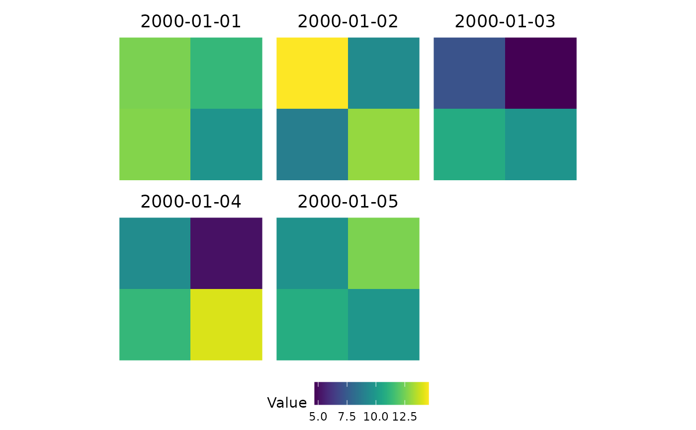A common legend across all panels can be enforced by setting common_legend = TRUE, which scales the fill range to the global minimum and maximum of the entire dataset.

Usage

nc_ggplot(
  data,
  title = FALSE,
  legend.title = NA,
  common_legend = FALSE,
  viridis.option = "viridis",
  ...
)

Arguments

data

An sxts object or a raster Raster* object (RasterLayer, RasterStack, RasterBrick).

title

Logical; if TRUE, layer names are added as plot titles. Default FALSE.

legend.title

Character; title for the colour legend. Use NA to omit. Default NA.

common_legend

Logical; if TRUE, a single common legend is collected across all panels with fill scaled to the global data range. Default FALSE.

viridis.option

Character; the viridis colour palette option ("viridis", "magma", "plasma", etc.). Default "viridis".

...

Additional arguments passed to wrap_plots.

Value

A ggplot2 object representing the raster map.

Examples

# Synthetic sxts with 4 cells and 5 daily steps
set.seed(42)
n <- 5
dates <- seq(as.POSIXct("2000-01-01", tz = "UTC"), by = "day", length.out = n)
vals <- matrix(rnorm(n * 4, mean = 10, sd = 2), nrow = n, ncol = 4)
coords <- data.frame(x = c(0, 1, 0, 1), y = c(0, 0, 1, 1))
ts_sxts <- sxts(data = vals, order.by = dates, coords = coords,
                projection = "+proj=longlat +datum=WGS84")

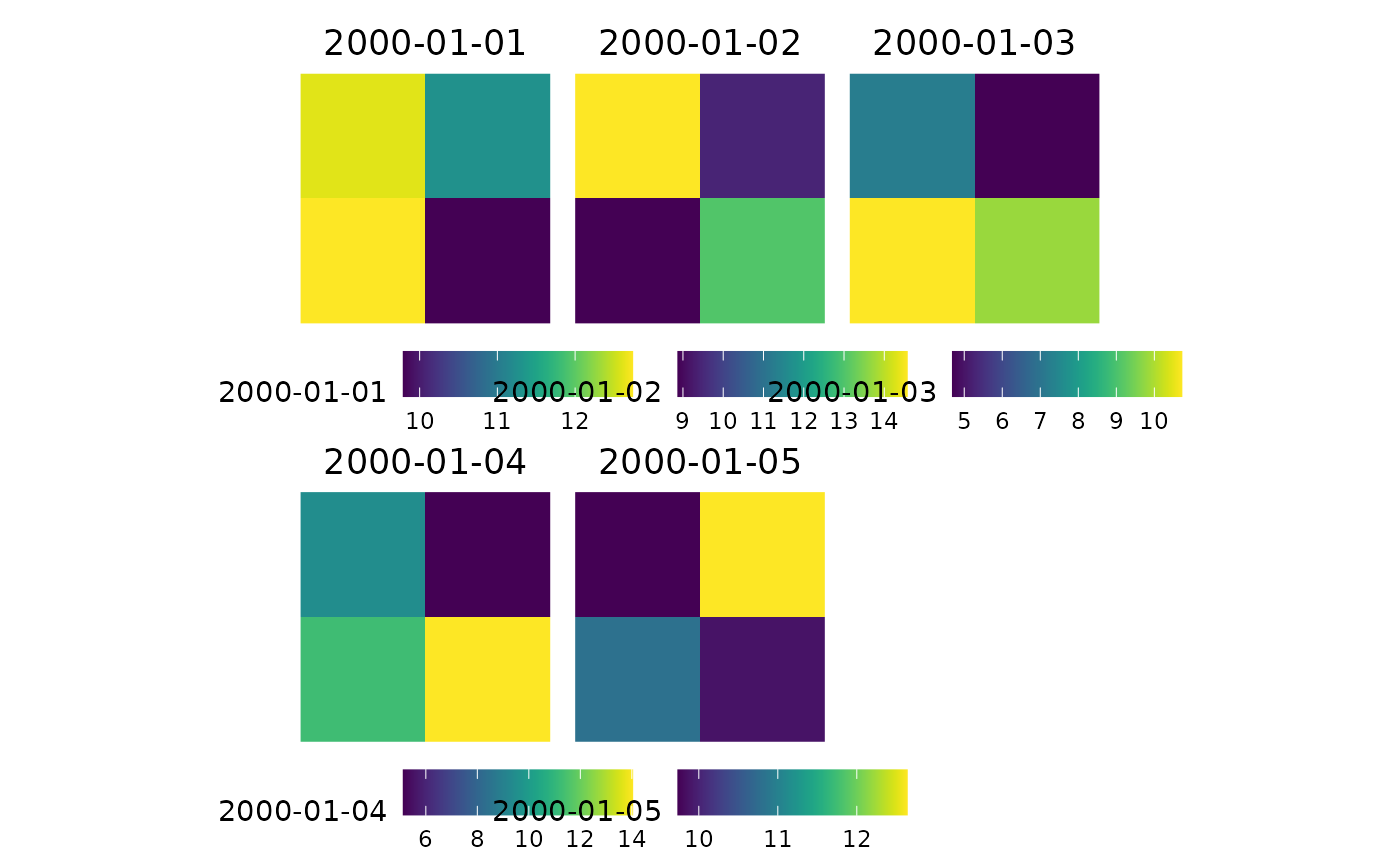
nc_ggplot(ts_sxts, title = TRUE)


# With a common legend
nc_ggplot(ts_sxts, title = TRUE, common_legend = TRUE,
          legend.title = "Value")