Diagnostics for a Fitted Distribution

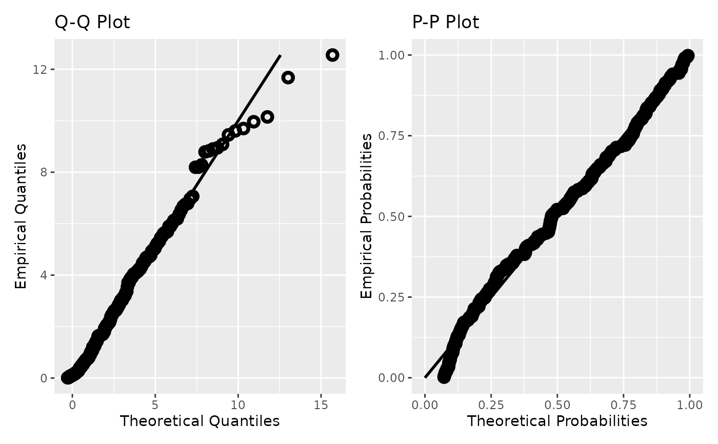
Produces diagnostic Q-Q and P-P plots together with two-sample goodness-of-fit statistics for a distribution previously fitted to a time series. The empirical quantiles are plotted against the theoretical quantiles computed from the supplied parameter list via the distribution's quantile function; the empirical cumulative probabilities are likewise compared with the theoretical CDF values in the P-P panel. Two-sample Cramér-von Mises and Kolmogorov-Smirnov statistics are computed on the empirical and fitted quantile vectors using pre-sorted, allocation-free routines. An optional zero-ignoring step filters values below a user-supplied threshold before constructing the diagnostic plots. The returned list contains the combined diagnostic panel, the individual Q-Q and P-P ggplot objects, and a GoF summary.

Usage

fit_diagnostics(
  ts,
  dist = "norm",
  params,
  ignore_zeros = FALSE,
  zero_threshold = 0.01
)

Arguments

ts

An xts object containing the time series data.

dist

A character string naming the distribution, e.g. "gamma3".

params

A named list of the fitted distribution parameters.

ignore_zeros

A logical value, if TRUE zeros will be ignored. Default is FALSE.

zero_threshold

The threshold below which values are considered zero. Default is 0.01.

Value

A list with components Diagnostic_Plots (a combined Q-Q and P-P panel via patchwork::wrap_plots), GoF (a named list of Cramér-von Mises and Kolmogorov-Smirnov statistics), QQplot, and PPplot (the individual ggplot objects).

Examples

# Daily precipitation-like data: gamma-distributed with zeros
x <- xts::xts(rgamma(365, shape = 0.8, scale = 3),
         order.by = seq.Date(as.Date("2020-01-01"), by = "day", length.out = 365))
x[sample(1:365, 100)] <- 0

fit <- fitlm_multi(x, candidates = 'gamma3', ignore_zeros = TRUE)
fcheck <- fit_diagnostics(x, dist = 'gamma3',
                          params = fit$parameter_list[[1]]$Param,
                          ignore_zeros = TRUE)
fcheck$Diagnostic_Plots